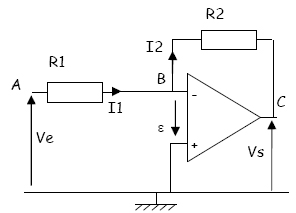
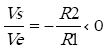
In the configuration shown here, the feedback is negative : the linear functioning is hence possible . How can we calculate the amplication Vs/Ve ? We use the model of the ideal op-amp : I+ = I- = 0 A=infinite, so if Vs does not reach its saturation values, the functioning is linear and ε = Vs/A = 0.
Consequently : V+ = V- = 0 I1 = I2 since I- = 0 Hence, we can write : Ve – V- = R1 . I1 = Ve Vs - V- = - R2. I2 = - R2. I1 = Vs	NB : We say that the point B is a virtual ground. B is a ground for the voltage, but it is an open circuit for the current. Indeed, the voltage V- at point B is zero as is the ground voltage, but there is no current between B and the ground, which is different from a real ground.

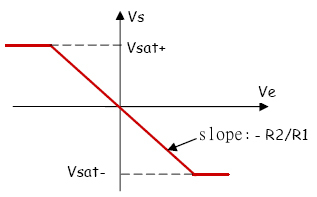
The signs of Vs and Ve signals are opposed, so the amplifier configuration is “inverting”.

This relationship Vs(Ve) is valid only as long as Vs has not reached its saturation values.

Characteristics of the inverting configuration :  Vs and Ve have opposed signs Vs amplitude can be greater, equal or less than Ve amplitude Input resistance : Re = Ve/ I1 = R1 Output resistance : Rs = 0